When it comes to evaluating a trading strategy, there are many ways people come to a conclusion on whether they think it will work or not.
There are Sharpe Ratios, Profit Factors, and more.
In this post today, we are going to break down how we evaluate a trading strategy here at Riskcuit.
This is by no means to say that this is the only way it should be done, or that this is the best way it can be done. This is just how we do it, and it works for us.
The goal of doing it this way is to calculate how many pips we can expect to make for every trade taken.
Before we really dig into though, there are a couple of main ideas we need to get across.
Everything Is A Distribution
The first big idea we want you to understand is, It doesn’t matter what you are trading, at the end of the day, at its core, it’s ultimately a distribution of possible outcomes or results.
Whether you are betting on how tall your children will be, the color of their eyes, whether your favorite team will win their next game, or where the GBP/USD currency pair will be trading at the end of the week, all you are really doing is exposing yourself in some way, typically financially, to a distribution of possible outcomes.
Any and every time you make a trade, this is what you are doing at its core.
It’s crucial to recognize this because only once we do, can we evaluate whether or not something is a good decision to make over and over again.
If we can’t estimate and calculate the distribution of possible outcomes to the best of our ability for any trade we are contemplating making, there is no way to tell in advance whether or not it is going to be a trade worth taking.
And if you have any aspirations to make money trading, understanding this will have more of an impact on your results than anything.
Once you understand and accept that everything is a distribution, you then need to recognize that there are 2 types of distributions and they are
- Distributions that are Perfectly Random (Completely Efficient)
- And those that aren’t… (Not Completely Efficient)
If something is perfectly random, or completely efficient, this means that there is almost no way to consistently make OR consistently lose money over time by repeatedly exposing yourself to that distribution.
The simplest example of this is a perfectly fair coin. If a coin is perfectly fair, it doesn’t matter how much discipline you have, or how sharp your psychological skills are, it will be impossible to consistently make money speculating on whether or not the coin will land on heads or tails.
The only way you can consistently make or lose money trading the distribution of outcomes is if they are not perfectly random. And thankfully currency, stock, future, and option prices are not perfectly random.
The main point to grasp here is, if there is any edge to be had, it must show up in the distribution itself.
Let’s illustrate this below. Below we have a histogram of the 4 Hour candle returns of EUR/USD in pips plotted out. In that same graph, we overlay what this histogram should look like if prices were perfectly random or “normal”.
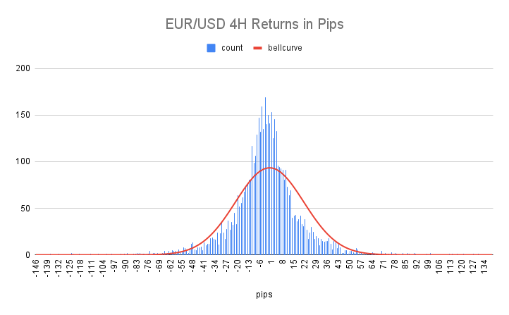
The first thing you can see is, the distribution of prices is clearly not normal. It’s very similar in shape, but it is not normal.
EUR/USD 4H candle returns are much more likely to be closer to 0 than is expected if they were normal. They are also much less likely to be in the ranges of -41 to – 10 and 10 – 41 than would be expected. And lastly, they are much more likely to be smaller than -62 or larger than 62 than what would be expected.
All this to say, the distribution is clearly fat-tailed.
For example, if the return of prices were truly random, the mean, median, and mode would all be 0. The skewness would be 0 and the kurtosis of prices would be 3.
In reality, though, the values for this distribution are:
- Mode: -3
- Median: -2
- Mean: -2.2998
- Skew: -0.05
- Kurtosis: 4.81
So we can clearly see that write off the bat, this distribution is NOT normal and it can be used to consistently generate profits.
However, this does not mean that the distribution right out of the box can be used to consistently generate profits. It does mean that it can be modified to do so though.
Modifying the Distribution of x
Next, we need to understand what entry and exit signals do to our distribution.
If you are taking a traditional buy-and-hold approach, where you bought EUR/USD, held your position for 4 hours, and closed once 4 hours had passed. The distribution of this system’s entries and exits would match the distribution of the price itself.
When we create entry and exit signals, we are essentially re-organizing the baseline distribution of price shown in our histogram above by slicing it up so we only observe certain values of x.
How to Evaluate Your System
Now that we understand that everything we trade is a distribution, and our entry and exit rules determine what that distribution looks like we can analyze whether or not a trading system or signal will work.
Using the same price distribution above, we will first look to see if applying our 4-hour buy-and-hold strategy directly to EUR/USD will prove to be profitable or not for us. In this example, we are only taking long trades.
To do this, we will walk through every possible value of x in the distribution and multiply it by the probability of that value of x occurring
We will then add together the result of each step of x.
This will result in the number of pips we can expect to make for every trade we take using this system.
Using the histogram above, this value results in -2.998 or essentially -3. So if we were to apply a buy-and-hold strategy on this distribution, we can expect to lose 3 pips on every position.
Let’s Change x
Now let’s apply some more rules to our system to change the distribution of x.
To keep it simple, we will set the following trading rules:
- If the price is above the 200 MA we will look to trade long and If the price is below the 200 MA we will look to trade short.
- We will use a fixed stop loss of 25 pips.
- We will close the trade after 24 candles have passed from our entry.
Apply these rules, this changes our histogram of x so that it looks like this:
It’s kind of hard to see what is happening here but what you should notice is our distribution looks completely different. The descriptive statistics for the distribution have also changed drastically:
- Mode: -25
- Median: -25
- Mean: 11.50
- Skewness: 1.9
- Kurtosis: 3.6
You can see by the kurtosis that this distribution of x is extremely fat-tailed. This means that most of the time we will see a value of -25 for x, and occasionally, we see really large positive values for x.
Just like we did previously, we will walk through every possible value of x in the distribution and multiply it by the probability of that value of x occurring
We will then add together the result of each step of x.
In this distribution, we end up with 11.
This means that with our entry and exit rules applied to the original distribution, we can expect to make 11 pips on any trade taken.
Again, if there is any edge in price that is to be taken advantage of, it must show up in the distribution itself.
Conclusion
This is how we evaluate systems at Riskcuit. I know it seems very complicated but once you understand it, it’s actually very simple and gives extremely accurate results.
It also allows you to see how you’re entry and exit signals change the distribution of x, allowing you to hone in and take advantage of a specific property of the original deviation.
In this example, we are focusing on the excess kurtosis of the original price distribution.
Remember, if the original price distribution’s characteristics deviate from what is expected in a normal distribution, you can use entry and exit signals to modify the distribution in order to take advantage of that discrepancy.
Sometimes the original price distribution can be used straight out of the box, but most times, you need to modify it.